It took me years before I understood exactly what a convolution is in the machine learning context. I understood the simple "filter moving over an image" convolution, but I couldn't figure out how to translate that into the operation that's performed by machine learning.
I read posts that used complex 4D diagrams (3D plus animation!) or 6-deep
nested for loops. Nothing against that if it makes sense to you, but it
never did to me.
It turns out there's a simple transformation from a basic convolution to an ML convolution. I haven't seen it explained this way anywhere else, so this is what I want to show in this post. Maybe it will help you like it helped me.
As a bonus, I'll show how this perspective makes it straightforward to observe the fact that 1x1 ML convolutions are just matrix multiplications.
Basic Convolutions
To review, a "basic convolution" is a function which takes as input two 2D arrays of real numbers:
- the "image", with dimensions
- \( H_i \) — input height
- \( W_i \) — input width, and
- the "filter" (also known as the "kernel"), with dimensions
- \( H_f \) — filter height
- \( W_f \) — filter width.
We expect the filter to be smaller than the image.
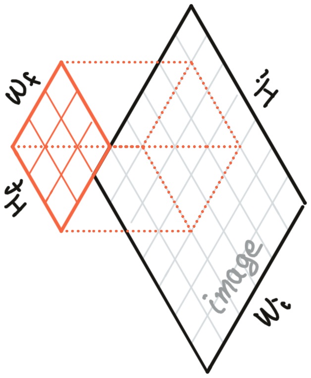
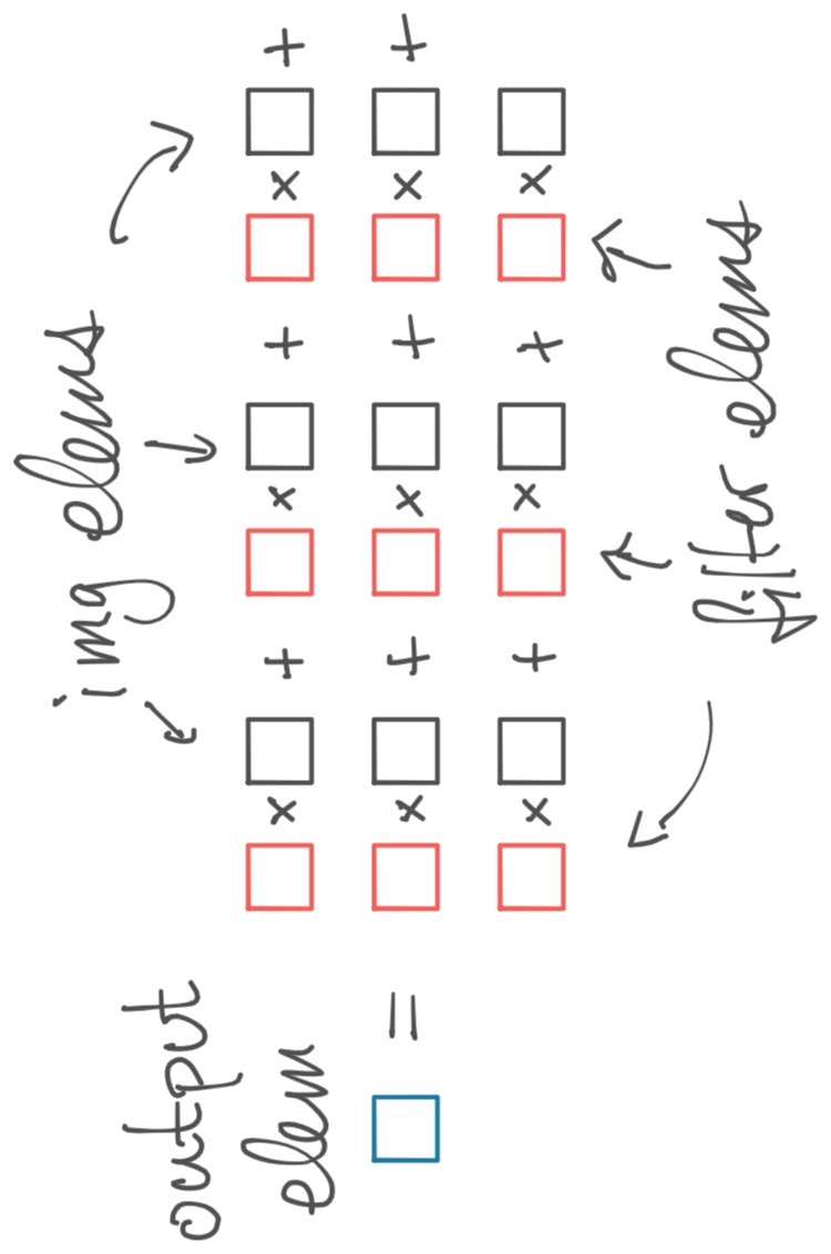
The basic convolution drags the filter over the image. At each point of overlap, we produce one output element by multiplying the values in the filter by the values in the image that are "beneath" them and adding up these products.
When the filter is in the top left of the input image, this process produces the top-leftmost output point. If the filter moves (say) one element rightward, we now generate the output point one element to the right from the top-left.
We thus produce an output image of size \( (H_o, W_o) \) (output height/width). The output is a little smaller than the input image because the kernel can't exceed the bounds of the input. (You can fix this by padding the input with 0s around the edges.)
To make up some notation describing the dimensions of the input/output arrays, we might write
\[ \operatorname{ConvBasic}( (H_i, W_i),\ (H_f, W_f) ) \rightarrow (H_o, W_o). \]
If you're not familiar with all this, check out this explainer, up to but not including the section entitled "the multi-channel version".
ML Convolutions
The basic convolution is simple enough. But an "ML convolution" is a different beast.
An ML convolution is an operation which operates on 4D arrays of real numbers.
- Input 1: the "image", with dimensions
- \( N \) — batch
- \( H_i \) — input height
- \( W_i \) — input width
- \( C_i \) — input channels,
- Input 2: "filter", with dimensions
- \( H_f \) — filter height
- \( W_f \) — filter width
- \( C_i \) — input channels
- \( C_o \) — output channels, and
- Output: the "output image", with dimensions
- \( N \) — batch
- \( H_o \) — output height
- \( W_o \) — output width
- \( C_o \) — output channels.
We can write this in our notation from above as
\[ \operatorname{MLConv}( (N, H_i, W_i, C_i),\ (H_f, W_f, C_i, C_o) ) \rightarrow (N, H_o, W_o, C_o). \]
Yikes, that's a lot of dimensions. What do they all mean, and how do they interact?
That's what I want to break down in this post. We'll take \( \operatorname{ConvBasic} \) and add one dimension at a time, until we have the full \( \operatorname{MLConv} \) function.
Input Channels
First, let's add input channels to the image.
Consider the elements of the image. Instead of them being real numbers, suppose they're vectors in \( \mathbb{R}^n \). For example, maybe your image is RGB; in this case, \( n=3 \). Or maybe your image is the result of an intermediate layer in a convolutional net; in this case, maybe \( n=128 \).
How do we "multiply" the elements of the image by the filter? One option is to let the elements of the filter also be vectors in \( \mathbb{R}^n \). Now when we multiply an element of the input by an element of the filter, we take their dot product, giving us a real number. Then like before, we add up all these dot products to get the output element, which is also a real number.
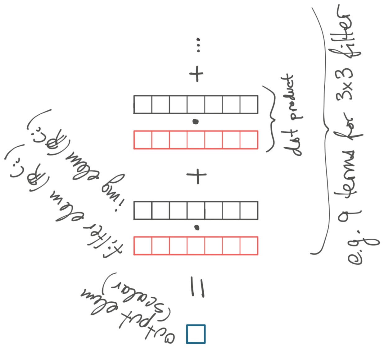
As you might have guessed, \( n \) is called the number of "input channels". It corresponds to dim \( C_i \).
So now we have a function which takes as input two 2D arrays, of size \( (H_i, W_i) \) and \( (H_f, W_f) \), where each element is a vector in \( \mathbb{R}^{C_i} \). Or equivalently, we take two 3D arrays of real numbers, of dimensions \( (H_i, W_i, C_i) \) and \( (H_f, W_f, C_i) \).
This operation still outputs a 2D array of real numbers of size \( (H_o, W_o) \), where the output height/width are a bit smaller than the input.
In our notation, this is
\[ \operatorname{ConvInputChannels}( (H_i, W_i, C_i),\ (H_f, W_f, C_i) ) \rightarrow (H_o, W_o). \]
Output Channels
Above, our output image is only 2D. Let's add the \( C_o \) ("output channels") dimension to make it 3D.
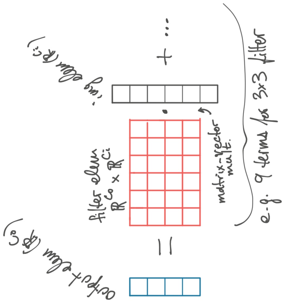
Suppose we create \( C_o \) independent filters and repeat the process above once for each filter. This results in \( C_o \) 2D output images.
Now the output is a 3D array of dimension \( (H_o, W_o, C_o) \). The filter also gains an additional dimension, \( (H_f, W_f, C_i, C_o) \).
Notice that we take the dot product of each element of the input image, a vector in \( \mathbb{R}^{C_i} \), with \( C_o \) different vectors from the filter. You can think of this as taking a repeated dot product, or equivalently as a matrix-vector multiplication.
In our notation, we now have
\[ \operatorname{ConvInOutChannels}( (H_i, W_i, C_i),\ (H_f, W_f, C_i, C_o) ) \rightarrow (H_o, W_o, C_o). \]
Batch Dimension
The only remaining dimension to handle is the "batch" dimension \( N \).
To add this, we have \( N \) independent input images which generate \( N \) independent output images. This is the batch dimension.
Now each output element is a \( (C_o, N) \) matrix, the sum of matrices formed by multiplying a \( (C_o, C_i) \) filter element by a \( (C_i, N) \) matrix.
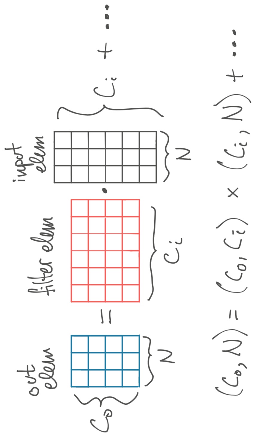
As before, we repeat this process for each of the \( H_o, W_o \) output elements.
We now have all four dimensions, so we can properly call this \( \operatorname{MLConv} \):
\[ \operatorname{MLConv}( (N, H_i, W_i, C_i),\ (H_f, W_f, C_i, C_o) ) \rightarrow (N, H_o, W_o, C_o). \]
Notice that the only difference between these four functions is in how we "multiply" elements.
- In \( \operatorname{ConvBasic} \) we multiply two scalars.
- In \( \operatorname{ConvInputChannels} \) we multiply two vectors.
- In \( \operatorname{ConvInOutChannels} \) we multiply a matrix and a vector.
- Finally, in \( \operatorname{MLConv} \) we multiply two matrices.
That's all an ML convolution is!
1x1 Convolutions
Now for our bonus fact. Suppose the filter's height and width are 1 — i.e. \( H_f = W_f = 1 \). I claim that this convolution is just a matrix multiplication.
First, observe that the batch, image height, and image width dimensions are interchangeable in a convolution with a 1x1 filter. That is, because there's no "mixing" along the height/width, we can reshape a \( (N, H_i, W_i, C_i) \) input into \( ( N \times H_i \times W_i, 1, 1, C_i ) \), do the conv, and then reshape back to the desired output shape.
So it's sufficient to show that a conv with 1x1 filter and input height/width 1 is a matmul.
But look at the diagram for "Batch Dimension" above. If the input height and width are 1, then there's only one output element. And if the filter size is 1x1, then there's only one term on the RHS, so the one output element is computed as a matmul. Thus, the whole operation is equivalent to a single matrix multiply! □
Thanks to George Karpenkov, Marek Kolodziej, Blake Hechtman, Kyle Huey, and Alexander Zinoviev for their feedback on drafts of this post.